
Note: All arc heights are in inches x 1000 - for example, 0.0054A is displayed as 5.4. The types of strip ( A, N or C) and exposure times (seconds, passes, rpm, etc) are not specified since these do not relate to this topic.
Investigation of a large data base resulted in the development of an equation that models the shape of Almen Saturation Curves. It was tested by tracing "perfect" data sets to confirm that results conform with current standards, common practice and experience.
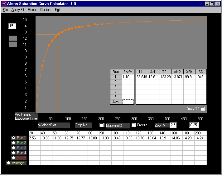
One such data set, generated using controlled production variables, was by Wieland(1). It consists of 388 Almen Strips shot-peened to saturation - and beyond - in fifteen time (exposure) increments. A plot of average arc heights and exposure times is shown below:
Fig. 1 15-point Data set (average of 30 sets consisting of 388 Almen strips)
Curve fit, with average of 99.9% (shown as %Fit above) and a Standard Deviation of .048 (.048/1000 or .000048 inch), is excellent. The curve itself displays characteristics that are familiar to all in the peen forming and shot peening field - a rapid initial vertical rise followed by a sharp "knee". After that, the vertical increase is at a much lesser rate but appears to continue in an indefinite straight line. This is the Almen Curve - exponential behavior and linear termination with a slope grater than zero - the y-intercept being close to, but not at, the saturation intensity.
The point of saturation itself is disclosed by visual inspection of the excellent data.
At T=60, data arc height is 12.25. At T=120, arc height is 13.78. Dividing the second arc height by the first yields:
T120/T60=13.78/12.25=1.125%
At T=70, data arc height is 12.77. At T=140 (not shown, the table above is scrolled to the left), it is 13.91.
T140/T70=13.91/12.77=1.089%
Optimum saturation exposure time is above T=60 and very close to T=70. The calculated T1=66.649 is valid. Even with excellent data sets, the difference in saturation exposure times translates into significant improvements in controlled shot peening as well as reductions in production times.
However, two questions must be answered:
1. Does the curve represent the true shape of Almen Saturation Curves?
2. Are similar results possible with less precise data?
The answers to both is yes!
If the equation models Almen Saturation Curves then, using only any two random data set points, one should be able to re-trace curves that duplicate the one in Fig. 1 above. Shown below, are re-trace overlays of the five 2-point sets. Succeeding plots essentially re-draw previous traces.
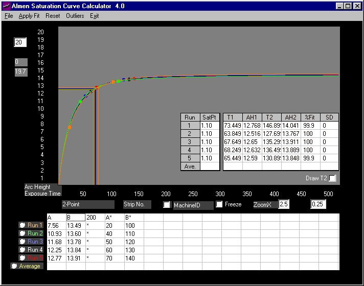
Fig. 2 Five 2-point data sets (from average values in Fig.1)
The five sets are recorded as Run1 to Run5 above. "A" and "B" are the exposure times that point to "A*" and "B*" on the right. For Run1 value of 7.56, "A" points to the exposure time of 20 on the right. For Run1 value of 13.49, "B" points to exposure time of 100 on the right. For Run2 value of 10.93, "A" points to the exposure time of 40 on the right ............. and so on.
There is one other number, 200. This is the exposure time of the last strip of the complete set. The software requires this to determine the sample size and anchor the data point location on the Almen Curve "time-universe" (arc height for exposure time 200 is not needed).
Saturation points of these sets are, for all practical purposes, the same as that calculated using fifteen strips. For 2-point sets, the goodness of fit should be 100%. Run1 and Run5 show a fit of only 99.9% - why? Some data sets require more time to analyze than others. By default, the software stops execution after a pre-set period of time - otherwise it could continue running indefinitely - at the conclusion of which, any improvements in calculated values may be meaningless (67.972 may improve to 67.972001 or 67.971999).
The curve drawn is valid. The saturation point was located using two reference points. Something like locating an object on a table by knowing how far it is from two adjacent sides - provided an accurate measuring tool is used.
Note: In order to draw saturation curves using only two Almen strips, the sample size must be known.
To know the sample size, all the strips have to be run. Results become more reliable and
reproducible in proportion to the number of Almen strips used and evaluated at any given Run.
The recommended minimum is four. The exercise above was simply to show that saturation
points are accurately located with Almen Saturation Curve Calculator 4.0.
The Wieland(1) raw data consists of 30 sets, the averages of which were used above. From these, five sets of 4-points, at exposure times of 20, 50, 100 and 200, are analyzed below.
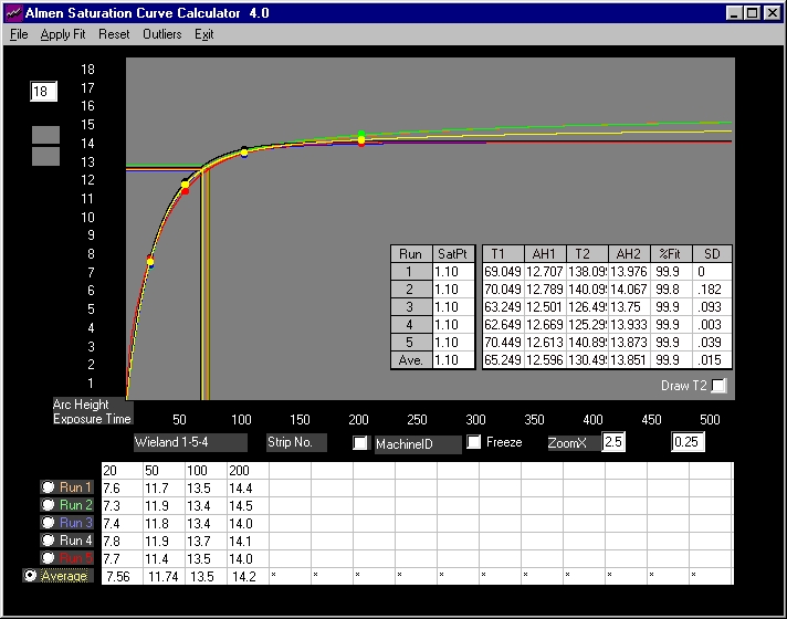
Fig. 3 Five 4-point data sets (from five 15-point sets, raw data)
Again, curves are drawn in overlays and individual data sets display excellent correlation. Average T1=65.249 is essentially the same as that from Fig. 1 (T1=66.649). Average AH1=12.596 is comparable to the AH1=12.611 from Fig.1. A tribute not only to the goodness of data but also to the accuracy of Almen Saturation Curve Calculator 4.0.
In the real world, running single 4-point sets is common practice particularly since, most often, it is undertaken to qualify approved setups prior to (and after) regular production runs. Below are two 4-point sets for WM320 1-2-4(2).
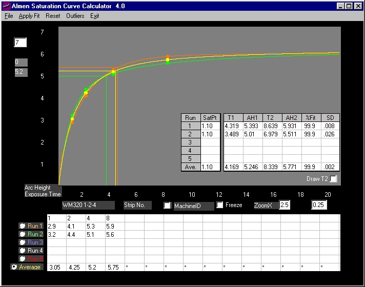
Fig. 4 Two 4-point sets Note: the asterisks are flags for data to be ignored - in this case, there is no data.
This is an example that illustrates another use of the calculator - to deliver accurate and verifiable information that is vital in decision-making, quality control and production.
The high correlation indicate that data represents the Almen Curve. The exposure times are in machine cycles. Visual inspection discloses that the saturation point from Run1 is between four and eight machine cycles (very much closer to four than eight). The calculator verifies AH1= 5.393 and T1=4.319 machine cycles - if fractional cycles cannot be run, this translates to 5 cycles (Arc Height >5.393 <5.931). It is difficult to infer saturation point for Run2 by visual inspection, it appears to be greater than 2 but less than 4 machine cycles . Starting from the origin (zero), the calculator goes up the curve until it discovers AH1=5.01 and T1=3.489. Again, this may translate into 4 machine cycles (Arc Height >5.01 <5.511). The average T1=4.169 (5 machine cycles Arc Height >5.246 <5.771) and the average AH1=5.246.
Variations in intensities are not great and would probably be acceptable. The difficult question is whether re-qualify production setup at four or five cycles (or to run another set of strips). The decision is entirely dependent on customer requirements, specifications and quality control.
For more details: peenforming@hotmail.com
References:
1. Wieland, R. C., "A Statistical Analysis of the Shot Peening Intensity Measurement", pp27-38,
Proceedings I.C.S.P.5, Oxford, 1993
2. Website peenforming.squarespace.com